demo20 of Im2mesh package
demo20 - 3d voxel image to tetrahedral mesh
Cite as: Ma, J., & Li, Y. (2025). Im2mesh: A MATLAB/Octave package for generating finite element mesh based on 2D multi-phase image (2.1.5). Zenodo. https://doi.org/10.5281/zenodo.14847059
Table of Contents
Gallery
Workflow
Dependencies
Installation of fTetWild via Docker
Initialize
STEP 1. Import 3d voxel image
STEP 2. Convert to triangular surface mesh
STEP 3. Smooth surface mesh
STEP 4. Select phases (optional)
STEP 5. Save surfaces as OFF file
STEP 6. Visualize surface mesh (optional)
STEP 7. Generate tetrahedral mesh via fTetWild
STEP 8. Assign phase labels & evaluate mesh quality
STEP 9. Visualize tetrahedral mesh
STEP 10. Export mesh as inp or bdf file
Export as bdf file (Nastran bulk data)
Export as inp file (Abaqus)
Troubleshooting
Mesh generation failure
Other issues
Gallery
Some examples created by me: https://mjx888.github.io/im2mesh_demo_html/gallery.html
Workflow
In Im2mesh demo20, the workflow of creating tetrahedral mesh is similar to the workflow in JM Hestroffer's XtalMesh ToolKit (see link below). The mesh generator of XtalMesh is fTetWild, which has very high meshing success rate due to its envelope-based meshing algorithm. Note that XtalMesh uses Python and cannot use 3d voxel image as input.
XtalMesh Github: https://github.com/jonathanhestroffer/XtalMesh
XtalMesh paper: https://doi.org/10.1007/s40192-022-00251-w
fTetWild Github: https://github.com/wildmeshing/fTetWild
fTetWild paper: https://dl.acm.org/doi/10.1145/3386569.3392385
fTetWild video: https://www.youtube.com/watch?v=RweR25IBeB8
I spent several days to rewrite XtalMesh's code to make it work for MATLAB and 3d voxel image. In this demo, we also use fTetWild as mesh generator.
Dependencies
To run demo20, we need to install fTetWild.
No need to install any MATLAB toolboxes.
Installation of fTetWild via Docker
2. Run Docker. If you have trouble in running Docker, you can ask AI for help. In my windows PC, I need to enable virtualization in BIOS to run Docker.
3. Open your command-line shell, such as Windows PowerShell.
4. Type the following code within command-line shell to install my Docker image of fTetWild (135.66 MB).
docker pull mjx0799/ftetwild
5. The installation may take a while (15-30 mins). After installation, your should be able to see the installed image in your Docker Desktop application.
Initialize
Before we start, open Docker Desktop application. Let it run in the background.
Open MATLAB, please set folder "Im2mesh_Matlab" as your current folder of MATLAB.
Clear variables.
clearvars
Set default image size (optional).
x = 250; y = 250; width = 250; height = 250;
set(groot, 'DefaultFigurePosition', [x,y,width,height])
% To reset:
% set(groot, 'DefaultFigurePosition', 'factory')
Define a subfolder for saving mesh data.
% Define the name of subfolder
folderName = 'myMesh';
myMeshFolder = fullfile(pwd, folderName);
% Creates the folder if it doesn't exist
if ~exist(myMeshFolder, 'dir')
mkdir(myMeshFolder);
disp('Folder created!');
end
STEP 1. Import 3d voxel image
We can import 3d image using function importImSeqs or function importImStack. We have demostrated these two functions in the beginning of demo19.
imageFoloder = 'test_image_sequences';
im = importImSeqs( imageFoloder );
Use function plotVolFaces to plot faces.
plotVolFaces( im );

We can use the function 'unique' to list all the grayscale intensity in the image.
unique(im)'
We can check the totoal number of grayscale intensity in the image.
length(unique(im))
ans = 4
Note that we identifies different phases in a image by their grayscales. Different grayscales correspond to different phases. If we have 4 level of grayscales in a image, the resulted meshes will contain 4 phases.
STEP 2. Convert to triangular surface mesh
We need to define the voxel spacing in the 3d voxel image. In the X-ray CT image of materials, the z spacing is usually different from the x and y spacing. We will set the actual phyiscal dimension of a voxel in STEP 10.
% Define the voxel spacing (default is 1x1x1)
voxelSpacing = [1.0, 1.0, 1.0];
We use function im2surf to convert 3d voxel image to 'blocky' triangular surface mesh. '[V, F, ntype, flabel]' is Dream.3D compatible format.
% 3d image to surface mesh
[V, F, ntype, flabel] = im2surf(im, voxelSpacing);
STEP 3. Smooth surface mesh
We will use constraint Taubin smoothing to smooth the 'blocky' triangular surface mesh. You can change 'num_iters' to tune surface smoothness. We can obtain smoother surface with a higher 'num_iters'. The typical value of 'num_iters' is 20-60.
For 3d image with a small size (100x100x100), you can try 'num_iters = 50;'.
For 3d image with a large size and very complex geometries, you can try 'num_iters = 30;'. In complex geometries, surface smoothing with 'num_iters = 50;' may induce some tangled triangles, potentially leading to mesh generation failure in STEP 7.
num_iters = 50;
lamda = 0.5;
mu = -0.53;
We use function smoothSurf to perform constraint Taubin smoothing. The smoothing process is the same as XtalMesh. You can check Figure 3 in JM Hestroffer's paper about the smoothing process. Note that XtalMesh used Laplacian smoothing, but I prefer Taubin smoothing (without volume shrinkage).
The smoothing process may take some time. Wait until "Smoothing Done!" show up.
% smooth surface
V = smoothSurf( V, F, ntype, num_iters, lamda, mu);
STEP 4. Select phases (optional)
The input 3d voxel image usually has multiple phases. Different grayscales in the image correspond to different phases.
grayscale = unique(im)'
We can use the following function the select the phases we desire. If we don't need to select phases, we can delete STEP 4 or set grayscale_we_like=[];
grayscale_we_like = [ 0, 134, 239 ];
[V, F, flabel] = selectPhase( V, F, flabel, grayscale_we_like );
STEP 5. Save surfaces as OFF file
Extract surfaces for each phase. We will use them later for phase labeling (STEP 8).
% Get surface mesh for each phase
phaseFaces = extractPhaseFaces(F, flabel);
We use function writeOFF to save surfaces as OFF file. We will send the OFF file to fTetWild in STEP 7.
offFileName = 'surface.off';
offFilePath = fullfile(myMeshFolder, offFileName);
writeOFF(offFilePath, V, F);
We can save these variables to mat file for backup.
save( 'surf.mat', 'V', 'F', 'phaseFaces' );
We may also save each phase's surface as OFF file. For visualizing surface mesh in other softwares.
numPhases = length(phaseFaces);
for i = 1:numPhases
% filename with a zero-padded integer
fileName = sprintf('surface_%02d.off', i);
writeOFF(fileName, V, phaseFaces{i});
end
We may also save each phase's surface as STL file. For visualizing surface mesh in other softwares.
numPhases = length(phaseFaces);
for i = 1:numPhases
[ Vtemp, Ftemp ] = delRedundantVertex( V, phaseFaces{i} );
TR = triangulation( Ftemp, Vtemp );
% filename with a zero-padded integer
fileName = sprintf('surface_%02d.stl', i);
stlwrite( TR, fileName, 'binary' );
end
clear Vtemp Ftemp TR
STEP 6. Visualize surface mesh (optional)
Matlab is really bad at plotting large data sets of surface mesh. I prefer using F3D to plot surface mesh via Command Line Interface. You may ask AI to generate some codes for plotting in F3D. You may also use Microsoft 3d Builder to check surface mesh.
In Matlab, we may use function plotSurface to visualize surface mesh.
color = 2;
opt = []; % reset
opt.faceAlpha = 0.5;
opt.sampleRatio = 1;
plotSurface( V, phaseFaces, color, opt );

If the input 3d image is large, function plotSurface could be very slow. I usually down-sample the surface to make the rendering faster. Down-sampling is achieved by setting 'opt.sampleRatio'.
'opt.sampleRatio = 1' means no down-sampling.
'opt.sampleRatio = 0.1' means roundly 10% down-sampling before plotting surface.
color = 1;
opt = []; % reset
opt.faceAlpha = 0.5;
opt.sampleRatio = 0.1;
plotSurface( V, phaseFaces, color, opt );

STEP 7. Generate tetrahedral mesh via fTetWild
To generate mesh via fTetWild, we need to construct a command and send the command to fTetWild via Docker.
There are 3 major parameters for fTetWild: Envelope size, Ideal edge length, and Filtering energy. Check out this image for the effect of these parameters on the generated mesh: https://mjx888.github.io/im2mesh_demo_html/fTetWild_parameter.jpg
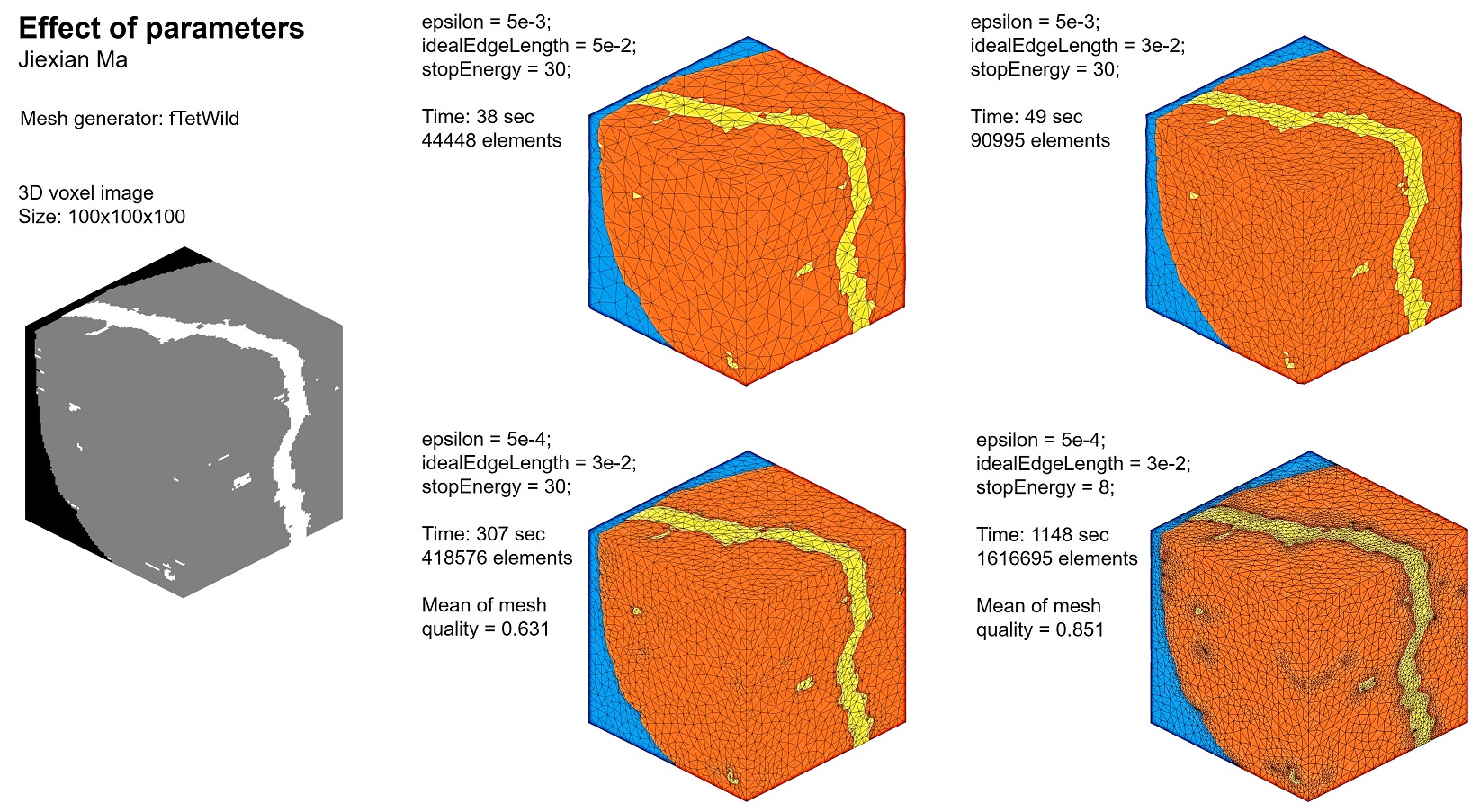
According to fTetWild, the meaning of these parameters is as follows.
Envelope of size epsilon: Using smaller envelope preserves fine features better but also takes longer time. The default value of epsilon is b/1000, where b is the length of the diagonal of the bounding box.
Ideal edge length: Using smaller ideal edge length gives a denser mesh but also takes longer time. The default ideal edge length is b/20, where b is the length of the diagonal of the bounding box.
Filtering energy: fTetWild stops optimizing the mesh when maximum energy is smaller than filtering energy. Thus, a smaller filtering energy means more optimization and better mesh quality, but takes longer time and generates more elements. If you do not care about quality, then setting a larger filtering energy would let you get the result earlier. The default filtering energy is 10. Range of filtering energy:3 to +inf. fTetWild suggest not to set filtering energy smaller than 8 for complex input.
According to fTetWild, we can use the following command line to set these parameters. For other command lines, see fTetWild's github page.
-e epsilon = diag_of_bbox * EPS. (double, optional, default: 1e-3)
-a Ideal edge length not scaled by diag_of_bbox. (double, optional)
-l ideal_edge_length = diag_of_bbox * L. (double, optional, default: 0.05)
--stop-energy Stop optimization when max energy is lower than this.
Command '-l ' is used to specify the scaled ideal edge length. You can use command '-a ' to specify the non-scaled ideal edge length. Command '-l ' and '-a ' are mutually exclusive (you cannot use both at the same time). For example, if the size of the input 3d image is 665x656x100, the bounding box diagonal length will be 939.447. If you set the scaled ideal edge length as 0.02, the non-scaled ideal edge length will be 0.02 x 939.447 = 18.79.
My suggestion for finding the optimal parameters is as follows. Suppose E is the envelope size, L is the scaled ideal edge length, and FE is the filtering energy.
- Start with large values, such as E = 5e-3, L = 5e-2, and FE = 30. Check the meshing result.
- Change L to a smaller value until you are satisfied.
- Keep the value of L constant. Reduce the value of E until the generated mesh can capture the fine features you desire.
- Keep the value of L and E constant. Set FE as 8 or 10. Generate mesh and check the mesh quality using function tetcost.
- If mesh generation fail, please refer to the end of this document (Troubleshooting section).
- If the mesh is too dense, increase E, L,or FE to reduce mesh density.
You may find that the generated mesh doesn't exactly conform to the input surfaces. For example, the boundary surfaces in the tetrahedral mesh are not flat, which can cause troubles when applying boundary conditions. To solve this, please refer to the Troubleshooting section.
The following code is an example of constructing a Docker command. The input is .off file. The output is .msh file (Gmsh format). You may ask AI to construct a Docker command.
epsilon = 5e-3; % Envelope size
idealEdgeLength = 5e-2; % Ideal edge length
stopEnergy = 10; % Filtering energy
mshFileName = 'tet.msh';
% Construct the Docker Command
dockerCmd = [
'docker run --rm -v "', myMeshFolder, ':/data" -w /data mjx0799/ftetwild ' ...
'--input ', offFileName, ' ' ...
'--output ', mshFileName, ' ' ...
'-e ', num2str(epsilon), ' ' ...
'-l ', num2str(idealEdgeLength), ' ' ...
'--stop-energy ', num2str(stopEnergy), ' ' ...
'--use-floodfill ' ...
'--manifold-surface ' ...
'--no-color ' ...
];
We use function genTet to send the command to fTetWild. After tetrahedral mesh is generated, we will see a .msh file (Gmsh format) in the subfolder we created before. Function genTet will automatically load the .msh file into MATLAB using sub-function readMsh.
The mesh generation process is very time-consuming. For example, on my old PC, when the size of the input 3d image is 665 x 656 x 100, E = 5e-3, L = 5e-2, and FE = 30, the time taken is 311 sec. When E = 7e-4, L = 2e-2, and FE = 30, the time taken is 1453 sec. When E = 7e-4, L = 2e-2, and FE = 8, the time taken is 3052 sec.
mshFilePath = fullfile( myMeshFolder, mshFileName );
% generate tetrahedral mesh
[vert, ele] = genTet( dockerCmd, mshFilePath );
STEP 8. Assign phase labels & evaluate mesh quality
We use function labelTet to assign phase labels. Wait until "Labeling complete!" show up.
[vert, ele, tnum] = labelTet(vert, ele, phaseFaces, V);
We can save variables to mat file for backup.
save('tet.mat', 'vert', 'ele', 'tnum');
We got 3 variables: vert, ele, tnum
vert: Mesh nodes. It’s a Nn-by-3 matrix, where Nn is the number of nodes in the mesh. Each row of vert contains the x, y, z coordinates for that mesh node.
ele: Mesh elements. It’s a Ne-by-4 matrix, where Ne is the number of elements.. Each row in ele contains the indices of the nodes for that mesh element.
tnum: Label of phase. Ne-by-1 array, where Ne is the number of elements.
tnum(j,1) = k; means the j-th element belongs to the k-th phase.
We use function tetcost to check mesh quality (shape quality). The computation method used by the tetcost function is the same as that used by the MATLAB built-in meshQuality function.

tetcost(vert, ele);
Plot mesh quality.
Q = tetcost(vert, ele);
figure
histogram(Q, 'BinLimits', [0,1], 'EdgeColor', 'none')
xlabel( "Element Shape Quality", "fontweight", "b" )
ylabel( "Number of Elements", "fontweight", "b" )

STEP 9. Visualize tetrahedral mesh
We use function plotMesh3d to plot mesh.
If you find the generated mesh is strange or some of the tetrahedrons are missing, please refer to the end of this document (Troubleshooting section).
plotMesh3d(vert, ele, tnum);

Other settings.
color = 2;
opt = []; % reset
opt.faceAlpha = 0.5;
opt.edgeAlpha = 0.5;
plotMesh3d( vert, ele, tnum, color, opt );

Define cutting plane to check interior. You can ask AI to define more setting.
opt = []; % reset
opt.cutPlaneYZ = 15; % plot elements where x <= 15
plotMesh3d(vert, ele, tnum, 1, opt);

We can plot the mesh for one of the phases. For example, the 2nd phase.
index = 2;
ele_temp = ele( tnum == index, : );
[ vert_temp, ele_temp ] = delRedundantVertex( vert, ele_temp );
color = 4;
opt = []; % reset
opt.faceAlpha = 1;
opt.edgeAlpha = 0.3;
plotMesh3d( vert_temp, ele_temp, [], color, opt );

STEP 10. Export mesh as inp or bdf file
Set up scale.
% physical dimensions of a voxel in the image
dx = 1;
Scale node coordinates according to dx.
% scale node coordinates of linear elements
vert = vert * dx;
Export as bdf file (Nastran bulk data)
precision = 8;
file_name = 'test_3d.bdf';
printBdf3d( vert, ele, tnum, [], precision, file_name );
Export as inp file (Abaqus)
Please refer to the following link to learn more about exporting mesh: https://github.com/mjx888/writeMesh/blob/main/README.md
Linear element
ele_type = 'C3D4';
precision = 8;
file_name = 'test_linear.inp';
opt = []; % reset
opt.tf_printMaxMinNode = 0;
opt.tf_printInterfNode = 0;
printInp3d( vert, ele, tnum, ele_type, precision, file_name, opt );
Quadratic element
We use function insertNode to convert the linear elements to quadratic elements.
% vert2, ele2 define quadratic elements
[vert2, ele2] = insertNode3d(vert, ele);
Export
ele_type = 'C3D10';
precision = 8;
file_name = 'test_quadratic.inp';
opt = []; % reset
opt.tf_printMaxMinNode = 0;
opt.tf_printInterfNode = 0;
printInp3d( vert2, ele2, tnum, ele_type, precision, file_name, opt );
If you require other file formats, you can ask AI to write Matlab functions for you.
Troubleshooting
Mesh generation failure
Mesh generation failure can be attributed to several reasons:
(1) Tangled triangular surfaces. If the input 3d image has complex geometries, surface smoothing with 'num_iters = 50;' may induce some tangled triangles, which can cause mesh generation failure. To fix this, go back to STEP 3 (Smooth surface mesh) and use a smaller value of 'num_iters'.
(2) Potential bugs of fTetWild. You can change the input parameters of fTetWild and run again.
(3) fTetWild terminated before the actual mesh generation process. This usually happens when the input 3d image has large size and has complex geometries. The failure is related to running out of RAM when fTetWild simplifies the large input surface mesh. You may use a PC with larger RAM to overcome this problem.
Other issues
Q1. Triangular surface mesh remains rough after surface smoothing (STEP 3). Increasing 'num_iters' fails to smooth the surface mesh further.
A1: I found this happens when the input 3d image has large size. The low-fequency noise in the triangular surface mesh remains after Taubin smoothing. You may try one of the following ways to solve this:
Method #1. Use rough surfaces as input for fTetWild, and set a larger value for the envelope of size epsilon. fTetWild will simplify the suface according to the giving epsilon, which can filter low-fequency noise.
Method #2. Aggressive smoothing by setting lamda = 0.90, mu = -0.91, num_iters = 100 (or larger value). Because the values of lamda and mu are close to 1.0, the algorithm is moving vertices nearly the maximum allowed distance during both the shrinking and inflating steps.
Advantages: Faster low-frequency reduction; Computational efficiency.
Disadvantages: High risk of instability; Self-intersection artifacts.
Q2. The boundary of the triangular surface mesh is pinned during surface smoothing (STEP 3). In some cases, we may prefer un-pinned boundary.
A2: This is due to the smoothing algorithm of XtalMesh. When the surface mesh touch the boundary (such as x-min & x-max), the surface mesh will be pinned at these location. We can add padding to the input 3d image to achieve un-pinned boundary.
Q3. fTetWild takes long time to generate mesh
A3: I'm aware that this is caused by the size of the input surface mesh. fTetWild struggles to simplify the surface mesh before mesh generation. This problem may be resolvable by using Matlab built-in function reducepatch to simplify surface mesh. Function reducepatch is faster in some cases. Feel free to contact me if you need help with this.
Q4. In the generated tetrahedral mesh, the mesh doesn't exactly conform to the input surfaces. For example, the boundary surfaces (such as x-min & x-max) in the tetrahedral mesh are not flat, which can cause troubles when applying boundary conditions.
A4: This is due to the envelope-based meshing algorithm of fTetWild. I have developed some code to fix this issue. Feel free to contact me if you need help with this.
Q5. How to actively terminate fTetWild during mesh generation?
A5: Open Docker desktop. In the Container Tab, we can actively terminate fTetWild.
Q6. Encounter the following error when using fTetWild via Docker.
docker: Error response from daemon: failed to create task for container
A6: Something is wrong in the constructed docker command.
If using docker image mjx0799/ftetwild, an example docker command is as follows.
dockerCmd = [
'docker run --rm -v "', myMeshFolder, ':/data" -w /data mjx0799/ftetwild ' ...
'--input ', offFileName, ' ' ...
'--output ', mshFileName, ' ' ...
'-e ', num2str(epsilon), ' ' ...
'-l ', num2str(idealEdgeLength), ' ' ...
'--no-color ' ...
];
If using docker image mjx0799/my_ftetwild_image, an example docker command is as follows.
dockerCmd = [
'docker run --rm -v "', myMeshFolder, ':/data" -w /data mjx0799/my_ftetwild_image ' ...
'/fTetWild/build/FloatTetwild_bin ' ...
'--input ', offFileName, ' ' ...
'--output ', mshFileName, ' ' ...
'-e ', num2str(epsilon), ' ' ...
'-l ', num2str(idealEdgeLength), ' ' ...
'--no-color ' ...
];
Q7. What is the difference between these two docker image: mjx0799/ftetwild, mjx0799/my_ftetwild_image
A7: The major difference is the size. mjx0799/ftetwild takes 135 MB, while mjx0799/my_ftetwild_image takes 1.7 GB. mjx0799/ftetwild uses docker multi-stage build to achieve lightweight container. Besides, the docker command is slightly different between these two image. See Q6.
Q8. Encounter the following error when using fTetWild via Docker.
The following arguments were not expected: --epsr-tags
A8: The standard build of fTetWild does not support the '--epsr-tags' command, which is used to specify envelope size for each input faces. To use the '--epsr-tags' command, you need install this docker image mjx0799/ftetwild_exact, which has enbled exact envelope. The drawback of fTetWild with exact envelope is the slow run time.
% reset image size
set(groot, 'DefaultFigurePosition', 'factory')
% end of demo